• Introduction
• Denoising Diffusion Probabilistic Model (DDPM)
• Forward Processs
  • Reverse Process
    • Loss function
      • Maximum Likelihood Learning.
      • Variational Lower Bound.
      • Training Loss Function \(\mathcal{L}_{\rm VLB}\).
      • Conditional Forward Transition Estimation.
      • Loss function parameterization.
  • Different Reparameterizations
    • X-space Reparameterization
    • V-space Reparameterization
• Appendix
  • Probability and Information Theory
    • Gaussian Distribution
      • Univariate Gaussian Distribution
      • Multivariate Gaussian Distribution
      • Isotropic Gaussian Distribution
    • Law of Large Number
      • Weak Law of Large Number
    • Entropy
    • Kullback-Leibler (KL) Divergence
      • General Form
      • Closed form for two Univariate Gaussian Distribution
    • Markov chain
  • Maximum Likelihood learning
  • Variational Lower Bound based Jensen’s Equality
  • Proof for \(p_\theta(x_{0:T}) = p(x_T)\prod_{t=1}^T p_\theta(x_{t-1}\mid x_t)\)
  • Proof for \(q(x_{1:T}\mid x_0) = \prod_{t=1}^T q(x_t\mid x_{t-1})\)

Introduction

Diffusion models have emerged as a powerful class of probabilistic generative models, demonstrating state-of-the-art performance in various machine learning tasks, particularly image synthesis. These models are grounded in the principles of stochastic processes, leveraging the concepts of forward and reverse diffusion to model data distributions. Diffusion models operate by progressively adding noise to data (forward diffusion) until it becomes a simple distribution, typically Gaussian. The reverse diffusion process then learns to denoise this noisy data back to its original form. This technical report provides an in-depth analysis of diffusion models, covering their theoretical underpinnings, algorithmic implementations, and practical applications. It is inspired by Lilian Weng’s comprehensive blog post “What are Diffusion Models?”, which offers a detailed and accessible explanation.

Denoising Diffusion Probabilistic Model (DDPM)

Diffusion models (DDPM) are latent variable models which have the form as follows:

\[\begin{align} p_\theta(x_0) = \int{p_\theta(x_{0:T})dx_{1:T}}, \end{align}\]

which is also the probability the generative model assigns to the data, \(x_1, \dots, x_T\) are latent vectors of the same dimensionality as the original data \(x_0 \sim q(x_0)\), as the prior distribution. Otherwise, \(\theta\) is the model parameter, \(T\) is the total number of timesteps in the Markov chain process.

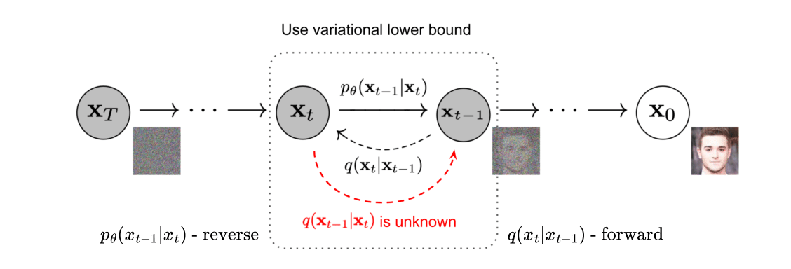
The idea behind DDPM is to gradually remove noise from a data sample (forward process), making it clearer step by step (reverse process). The underlying issue is how to approximate the transition from noise back to the original data point. This technical report will undercover mathematically both forward and reverse processes, especially in the reverse process the loss function construction, conditional forward transition estimation, and its parameterized version.

Forward Processs

Diffusion models(DDPM) use of a specific approximate posterior, \(q(x_{1:T} \mid x_0)\), known as the forward process or diffusion process. This process is predetermined as a Markov chain that incrementally introduces Gaussian noise to the sample in \(T\) steps, following a predefined variance schedule \(\beta_1, \ldots, \beta_T\) as \(\beta_t \in (0, 1)\) for \(t = 1, \ldots, T\).

\[\begin{align} q(x_{1:T} \mid x_0) = \prod_{t=1}^{T} q(x_{t} \mid x_{t-1}), \end{align}\] \[\begin{align} q(x_{t} \mid x_{t-1}) = \mathcal{N}(x_t;\sqrt{1-\beta_t}x_{t-1}, \beta_t\textbf{I}) \end{align}\]

The intuition behind \(\sqrt{1-\beta_t}\) is that authors(DDPM) would like to keep the latent variance in all timestep constant, specifically to 1. Considering an unknown variance across timesteps \(\nu_t\), hence the density of \(x_t\) conditioned on \(x_{t-1}\) is as follows:

\[\begin{align} q(x_{t} \mid x_{t-1}) = \mathcal{N}(x_t;\nu_t x_{t-1}, \beta_t\textbf{I}) \end{align}\]

The variance of \(x_t\) is as follows:

\[\begin{align}\label{eq:var_x_t} Var[x_t] &= Var\left[\nu_t x_{t-1} + \sqrt{\beta_t}\epsilon_t\right] \\ &= \nu_t^2Var\left[x_{t-1}\right] + \beta_tVar\left[\epsilon_t\right] + \nu_t^2\beta_tCov\left[x_{t-1}, \epsilon_t\right] \end{align}\]

Since \(p_{t-1}\) and \(p(\epsilon_t)\) are independent, thus \(p(x_{t-1}, \epsilon_t) = p(x_{t-1})p(\epsilon_t)\) and \(Cov[x_{t-1}, \epsilon_t] = 0\). Substituting into Equation \eqref{eq:var_x_t}, we have:

\[\begin{align} Var[x_t] &= Var\left[\nu_t x_{t-1} + \sqrt{\beta_t}\epsilon_t\right] \\ &= \nu_t^2 Var\left[x_{t-1}\right] + \beta_t Var\left[\epsilon_t\right] \\ &= \nu_t^2 Var\left[x_{t-1}\right] + \beta_t \quad\textrm{since $\epsilon\sim\mathcal{N}(0, \textbf{I})$} \end{align}\]

Given that, we would like the variance of latent across timesteps to be \(1\), so we set \(Var[x_t] = Var[x_{t-1}] = 1\), we have

\[\begin{align} 1 &= \nu_t^2 + \beta_t\\ \Leftrightarrow \nu_t &= \sqrt{1 - \beta_t} \end{align}\]

As the time step \(T\) increases, the distinguishable features of the initial data sample \(x_0\) gradually diminish. As \(T\) approaches infinity, \(x_T\) converges to an isotropic Gaussian distribution. A beneficial aspect of this process is that it allows for sampling \(x_t\) at any chosen time step \(T\) in a closed form by utilizing the reparameterization trick (VAE).

\[\begin{align} x_t &= \sqrt{1-\beta_t}x_{t-1} + \sqrt{\beta_t}\epsilon_{t-1}; \quad \textrm{where} \quad \epsilon_{t-1}, \epsilon_{t-2},\ldots~ \mathcal{N}(0, \textbf{I})\\ &= \sqrt{\alpha_t}x_{t-1} + \sqrt{1-\alpha}\epsilon_{t-1}; \quad \textrm{where} \quad \alpha_t = 1 - \beta_t \quad and \quad \bar{\alpha} =\prod_{t=1}^{T}\alpha_i\\ &= \sqrt{\alpha_t \alpha_{t-1}}x_{t-2} + \sqrt{1- \alpha_t \alpha_{t-1}}\bar{\epsilon}_{t-2}; \quad\textrm{where} \quad\bar{\epsilon}_{t-2} \quad \textrm{ is merged two Gaussians(*)}\\ &= \ldots\notag\\ &= \sqrt{\bar\alpha_t}x_0 + \sqrt{1- \bar\alpha_t}\epsilon \end{align}\]

As a result,

\[\begin{align} q(x_{t} \mid x_{0}) = \mathcal{N}(x_t;\sqrt{\bar\alpha_t}x_0, (1- \bar\alpha_t)\textbf{I}) \end{align}\]

Typically, a larger update step can be taken when the sample becomes noisier, so \(\beta_1 < \beta_2<\ldots< \beta_T\) and therefore \(\bar\alpha_1> \bar\alpha_2>\ldots>\bar\alpha_T\).

Reverse Process

The reverse process (refers to Equation \eqref{eq:rev}) is the joint distribution \(p_\theta(x_{0:T})\), defined as a Markov chain with learned Gaussian transitiion starting at \(p(x_T) = \mathcal{N}(x_T, 0, \textbf{I})\). By conducting the reverse process, the model will be able to recreate the true sample from a Gaussian noise input, \(x_T \sim \mathcal{N}(0, \textbf{I})\).

\[\begin{align}\label{eq:rev} p_\theta(x_{0:T}) = p(x_T)\prod p_\theta(x_{t-1}\mid x_t) \end{align}\]

The transition probability in the reverse process is then approximated by model \(\theta\) as follows:

\[\begin{align} p_\theta(x_{t-1}\mid x_t) = \mathcal{N}(x_{t-1}; \boldsymbol{\mu}_\theta(x_t, t), \boldsymbol{\Sigma}_\theta(x_t, t)) \end{align}\]

where the transition probability distribution is expected to be Gaussian distribution with mean and variance approximated by \(\boldsymbol{\mu}_\theta(x_t, t)\) and \(\boldsymbol{\Sigma}_\theta(x_t, t)\). Note that both \(\boldsymbol{\mu}_\theta\) and \(\boldsymbol{\Sigma}_\theta(x_t, t)\) are conditioned on \(t\), considered as a positional encoding or timestep guidance.

Loss function

Maximum Likelihood Learning.

DDPM(DDPM) objective function also minimizes the “closeness” between data distribution \(\log p_{\rm data}(x_0)\) and empirical estimated distribution \(p_\theta(x_0)\) as VAEs(VAE), by maximizing the estimated entropy or negative log-likelihood (refers to Equation \eqref{eq:nlll}), which is detailedly derived at Section APXMLL.

\[\begin{align}\label{eq:nlll} \mathcal{L}(x_0) = -\mathbb{E}_{x_0\sim p_{\rm data}(x_0)}\log p_\theta(x_0) \end{align}\]

To sample the data through a Markov chain process, where each transition is a Gaussian distribution, the loss function needs to minimize the distribution distance between two transitions, which are forward transition and reverse transition. To minimize the distribution divergence between two transitions, DDPM(DDPM) uses KL-divergence as follows:

\[\begin{align} \mathcal{L}(q(x_{1:T}|x_0), p_\theta(x_{1:T}|x_0)) = \mathcal{D}_{\rm KL}(q(x_{1:T}|x_0)\|p_\theta(x_{1:T}|x_0)) \end{align}\]

Given that KL-divergence is a positive value function, the upper bound of the negative log-likelihood is then obtained as follows:

\[\begin{align} 0 &\leq \mathcal{D}_{\rm KL}(q(x_{1:T}|x_0)\|p_\theta(x_{1:T}|x_0)) \\ -\log p_\theta(x_0) &\leq -\log p_\theta(x_0) + \mathcal{D}_{\rm KL}(q(x_{1:T}|x_0)\|p_\theta(x_{1:T}|x_0)) \end{align}\]

Variational Lower Bound.

Based on VAE(VAE) setup, the loss function is the negative log-likelihood optimized by a variational lower bound (refers to Equation \eqref{eq:diff-lvb}). The entropy of the input data \(\mathcal{H}(x_0) = -\log p_\theta(x_0)\) now has the upper bound, presented in the last equal sign. The reverse process loss function then minimizes this upper bound (variational lower bound can be proven using Jensen’s equality at Section Variational Lower Bound based Jensen’s Equality).

\[\begin{align}\label{eq:diff-lvb} -\log p_\theta(x_0) &\leq -\log p_\theta(x_0) + \mathcal{D}_{\rm KL}(q(x_{1:T}|x_0)\|p_\theta(x_{1:T}|x_0)) \\ &=-\log p_\theta(x_0) + \mathbb{E}_{x_{1:T}\sim q(x_{1:T}|x_0)}\log\frac{q(x_{1:T}|x_0)}{p_\theta(x_{1:T}|x_0)} \\ &=-\log p_\theta(x_0) + \mathbb{E}_{x_{1:T}\sim q(x_{1:T}|x_0)}\log\frac{q(x_{1:T}|x_0)}{p_\theta(x_{1:T},x_0)/p_\theta(x_0)} \\ &=-\log p_\theta(x_0) + \mathbb{E}_{x_{1:T}\sim q(x_{1:T}|x_0)}\log\frac{q(x_{1:T}|x_0)}{p_\theta(x_{0:T})/p_\theta(x_0)} \\ &=-\log p_\theta(x_0) + \mathbb{E}_{x_{1:T}\sim q(x_{1:T}|x_0)}\log\left[\frac{q(x_{1:T}|x_0)}{p_\theta(x_{0:T})}p_\theta(x_0)\right] \\ &=-\log p_\theta(x_0) + \mathbb{E}_{x_{1:T}\sim q(x_{1:T}|x_0)}\left[\log\frac{q(x_{1:T}|x_0)}{p_\theta(x_{0:T})} + \log p_\theta(x_0)\right] \\ &=-\log p_\theta(x_0) + \mathbb{E}_{x_{1:T}\sim q(x_{1:T}|x_0)}\left[\log\frac{q(x_{1:T}|x_0)}{p_\theta(x_{0:T})}\right] + \log p_\theta(x_0) \\ &=\mathbb{E}_{x_{1:T}\sim q(x_{1:T}|x_0)}\left[\log\frac{q(x_{1:T}|x_0)}{p_\theta(x_{0:T})}\right] \end{align}\]

Training Loss Function \(\mathcal{L}_{\rm VLB}\).

From Equation \eqref{eq:diff-lvb}, the training loss function is then expressed as follows:

\[\begin{align}\label{eq:vlb-upper} \mathcal{L}_{\rm VLB} &= \mathbb{E}_{q(x_{0:T})}\left[\log\frac{q(x_{1:T}|x_0)}{p_\theta(x_{0:T})}\right] \\ &= \mathbb{E}_{q(x_{0:T})}\left[\log\frac{\textcolor{blue}{\prod_{t=1}^T q(x_t|x_{t-1})}}{\textcolor{red}{p_\theta(x_T)}\textcolor{blue}{\prod_{t=1}^T p_\theta(x_{t-1}\mid x_t)}}\right] \end{align}\]

Based on Markov chain properties, the nominator and dominator of Equation \eqref{eq:vlb-upper} can be expressed as the product of conditional probabilities (The detailed proofs are refer to Equations \eqref{eq:vlb-proof:upper} and \eqref{eq:vlb-proof:lower}). Equation \eqref{eq:vlb-upper} can be expressed as follows:

\[\begin{align} \mathcal{L}_{\rm VLB} &= \mathbb{E}_{q(x_{0:T})}\left[\log\frac{1}{\textcolor{red}{p_\theta(x_T)}} + \log\textcolor{blue}{\frac{\prod_{t=1}^T q(x_t\mid x_{t-1})}{\prod_{t=1}^T p_\theta(x_{t-1}\mid x_t)}}\right] \\ &= \mathbb{E}_{q(x_{0:T})}\left[-\log p_\theta(x_T) + \sum_{t=1}^T\log\frac{q(x_t\mid x_{t-1})}{p_\theta(x_{t-1}\mid x_t)}\right] \\ &= \mathbb{E}_{q(x_{0:T})}\left[-\log p_\theta(x_T) + \sum_{t=2}^T\log\frac{\textcolor{teal}{q(x_t\mid x_{t-1})}}{p_\theta(x_{t-1}\mid x_t)} + \log\frac{q(x_1\mid x_0)}{p_\theta(x_0\mid x_1)}\right] \end{align}\]

Applying the Bayes’ Rule, the nominator can be expressed as follows:

\[\begin{align} \textcolor{teal}{q(x_t \mid x_{t-1})} = \frac{q(x_t, x_{t-1})}{q(x_{t-1})} = \frac{q(x_{t-1}\mid x_t)q(x_t)}{q(x_{t-1})} \end{align}\] \[\begin{align}\label{eq:vlb-norm-x0} \textcolor{teal}{q(x_t \mid x_{t-1}, x_0)} = \frac{q(x_t, x_{t-1}, x_0)}{q(x_{t-1}, x_0)} = \frac{q(x_{t-1}\mid x_t, x_0)q(x_t, x_0)}{q(x_{t-1}, x_0)} \end{align}\]

According to Denoising Diffusion Probabilistic Models (DDPM), \(\textcolor{teal}{q(x_t \mid x_{t-1})}\) is intractable, hence conditioning it with \(x_0\). Note that conditioning on \(x_0\) does not break the Bayes’ Rule (refers to Equation \eqref{eq:vlb-norm-x0}). The loss function \(\mathcal{L}_{VLB}\) can be expressed as follows:

\[\begin{align} \mathcal{L}_{\rm VLB} &= \mathbb{E}_{q(x_{0:T})}\left[-\log p_\theta(x_T) + \sum_{t=2}^T\log\frac{q(x_{t-1}\mid x_t)}{p_\theta(x_{t-1}\mid x_t)}\frac{q(x_t)}{q(x_{t-1})} + \log\frac{q(x_1\mid x_0)}{p_\theta(x_0\mid x_1)}\right] \\ &= \mathbb{E}_{q}\left[-\log p_\theta(x_T) + \sum_{t=2}^T\log\frac{q(x_{t-1}\mid x_t, x_0)}{p_\theta(x_{t-1}\mid x_t)}\frac{q(x_t\mid x_0)}{q(x_{t-1}\mid x_0)} + \log\frac{q(x_1\mid x_0)}{p_\theta(x_0\mid x_1)}\right] \\ &= \mathbb{E}_{q}\left[-\log p_\theta(x_T) + \sum_{t=2}^T\log\left(\frac{q(x_{t-1}\mid x_t, x_0)}{p_\theta(x_{t-1}\mid x_t)} + \log\frac{q(x_t\mid x_0)}{q(x_{t-1}\mid x_0)}\right) + \log\frac{q(x_1\mid x_0)}{p_\theta(x_0\mid x_1)}\right] \\ &= \mathbb{E}_{q}\left[-\log p_\theta(x_T) + \sum_{t=2}^T\log\left(\frac{q(x_{t-1}\mid x_t, x_0)}{p_\theta(x_{t-1}\mid x_t)} + \log\frac{q(x_t\mid x_0)}{q(x_{t-1}\mid x_0)}\right) + \log\frac{q(x_1\mid x_0)}{p_\theta(x_0\mid x_1)}\right] \\ &= \mathbb{E}_{q}\left[-\log p_\theta(x_T) + \sum_{t=2}^T\log\frac{q(x_{t-1}\mid x_t, x_0)}{p_\theta(x_{t-1}\mid x_t)} + \textcolor{red}{\sum_{t=2}^T\log\frac{q(x_t\mid x_0)}{q(x_{t-1}\mid x_0)}} + \log\frac{q(x_1\mid x_0)}{p_\theta(x_0\mid x_1)}\right] \end{align}\]

The second sum of logarithms can be shortened as follows:

\[\begin{align} \textcolor{red}{\sum_{t=2}^T\log\frac{q(x_t\mid x_0)}{q(x_{t-1}\mid x_0)}} &= \log\prod_{t=2}^T \frac{q(x_t\mid x_0)}{q(x_{t-1}\mid x_0)} \\ &= \log\frac{q(x_2\mid x_0)}{q(x_1\mid x_0)}\frac{q(x_3\mid x_0)}{q(x_2\mid x_0)}\dots\frac{q(x_{T-1}\mid x_0)}{q(x_{T-2}\mid x_0)}\frac{q(x_T\mid x_0)}{q(x_{T-1}\mid x_0)} \\ &= \textcolor{blue}{\log\frac{q(x_T\mid x_0)}{q(x_1\mid x_0)}} \end{align}\]

Substituting \(\sum_{t=2}^T\log(q(x_t\mid x_0)/q(x_{t-1}\mid x_0)) = \log(q(x_T\mid x_0)/q(x_1\mid x_0))\), we have:

\[\begin{align} \mathcal{L}_{\rm VLB} &= \mathbb{E}_{q}\left[-\log p_\theta(x_T) + \sum_{t=2}^T\log\frac{q(x_{t-1}\mid x_t, x_0)}{p_\theta(x_{t-1}\mid x_t)} + \textcolor{blue}{\log\frac{q(x_T\mid x_0)}{q(x_1\mid x_0)}} + \log\frac{q(x_1\mid x_0)}{p_\theta(x_0\mid x_1)}\right] \\ &= \mathbb{E}_{q}\left[\log\frac{q(x_T\mid x_0)}{p_\theta(x_T)} + \sum_{t=2}^T\log\frac{q(x_{t-1}\mid x_t, x_0)}{p_\theta(x_{t-1}\mid x_t)} -\log(p_\theta(x_0\mid x_1))\right] \\ &= \mathbb{E}_{q}\left[\underbrace{\mathcal{D}_{\rm KL}(q(x_T\mid x_0) \| p_\theta(x_T))}_{\mathcal{L}_T}+ \sum_{t=2}^T\underbrace{\mathcal{D}_{\rm KL}(\textcolor{red}{q(x_{t-1} \mid x_t, x_0)})\|p_\theta(x_{t-1}\mid x_t))}_{\mathcal{L}_{t-1}}-\underbrace{\log(p_\theta(x_0\mid x_1))}_{\mathcal{L}_0}\right] \label{eq:final-general-vlb} \end{align}\]

Conditional Forward Transition Estimation.

It is noteworthy that the reverse conditional probability is tractable when conditioned on \(x_0\) (refers to Equation \eqref{eq:vlb-norm-x0}). To estimate \(\textcolor{red}{q(x_{t-1} \mid x_t, x_0)}\), (DDPM) considers the probability as Gaussian distribution and tried to find \(\boldsymbol{\tilde{\mu}}(x_{t-1}, x_0)\) and \(\tilde{\beta}_t\).

\[\begin{align} q(x_{t-1} \mid x_t, x_0) \sim\mathcal{N}(x_{t-1}; \boldsymbol{\tilde{\mu}}(x_t, x_0), \tilde{\beta}_t\boldsymbol{I}) \end{align}\]

Applying the Bayes’ Rule and Markov chain, \(q(x_t\mid x_{t-1}, x_0)\) can be expressed as follows:

\[\begin{align} \mathcal{I} = q(x_{t-1} \mid x_t, x_0) = q(x_t\mid x_{t-1}, x_0)\frac{q(x_{t-1}\mid x_0)}{q(x_t\mid x_0)} = q(x_t\mid x_{t-1})\frac{q(x_{t-1}\mid x_0)}{q(x_t\mid x_0)} \end{align}\]

Given that the forward process is based on Gaussian distribution (refers to Equation ), hence \(\boldsymbol{\tilde{\mu}}(x_{t-1}, x_0)\) and \(\tilde{\beta}_t\) can be found by applying the probability distribution function.

\[\begin{align} \begin{cases} q(x_t\mid x_{t-1}) = \mathcal{N}(x_t; \sqrt{a_t}x_{t-1}, (1 - a_t)\textbf{I}) = (2\pi(1-a_t))^{-\frac{1}{2}}\exp{\Big\{\frac{(x_t - \sqrt{a_t}x_{t-1})^2}{-2(1-a_t)}\Big\}}\\ q(x_{t-1}\mid x_0) = \mathcal{N}(x_{t-1}; \sqrt{\bar{a}_{t-1}}x_0, (1 - \bar{a}_{t-1})\textbf{I}) = (2\pi(1-\bar{a}_{t-1}))^{-\frac{1}{2}}\exp{\Big\{\frac{(x_{t-1} - \sqrt{\bar{a}_{t-1}}x_0)^2}{-2(1-\bar{a}_{t-1})}\Big\}}\\ q(x_t\mid x_0) = \mathcal{N}(x_t; \sqrt{\bar{a}_t}x_0, (1 - \bar{a}_t)\textbf{I}) = (2\pi(1-\bar{a}_t))^{-\frac{1}{2}}\exp{\Big\{\frac{(x_t - \sqrt{\bar{a}_t}x_0)^2}{-2(1-\bar{a}_t)}\Big\}} \end{cases} \end{align}\]

Substituting \(q(x_t\mid x_{t-1})\), \(q(x_{t-1}\mid x_0)\), and \(q(x_t\mid x_0)\) into \(q(x_t\mid x_{t-1}, x_0)\), we have

\[\begin{align} \mathcal{I} &= (2\pi(1-a_t))^{-\frac{1}{2}}\exp{\Big\{\frac{(x_t - \sqrt{a_t}x_{t-1})^2}{-2(1-a_t)}\Big\}}\frac{(2\pi(1-\bar{a}_{t-1}))^{-\frac{1}{2}}\exp{\Big\{\frac{(x_{t-1} - \sqrt{\bar{a}_{t-1}}x_0)^2}{-2(1-\bar{a}_{t-1})}\Big\}}}{(2\pi(1-a_t))^{-\frac{1}{2}}\exp{\Big\{\frac{(x_t - \sqrt{a_t}x_0)^2}{-2(1-\bar{a}_t)}\Big\}}} \\ &\varpropto \exp{\left\{\frac{(x_t - \sqrt{a_t}x_{t-1})^2}{-2(1-a_t)}\right\}}\frac{\exp{\left\{\frac{(x_{t-1} - \sqrt{\bar{a}_{t-1}}x_0)^2}{-2(1-\bar{a}_{t-1})}\right\}}}{\exp{\left\{\frac{(x_t - \sqrt{a_t}x_0)^2}{-2(1-\bar{a}_t)}\right\}}} \\ &\varpropto \exp{\left\{\frac{(x_t - \sqrt{a_t}x_{t-1})^2}{(1-a_t)} + \frac{(x_{t-1} - \sqrt{\bar{a}_{t-1}}x_0)^2}{(1-\bar{a}_{t-1})} - \frac{(x_t - \sqrt{a_t}x_0)^2}{(1-\bar{a}_t)}\right\}} \\ &= \exp{\left\{\frac{x_t^2 - 2\sqrt{a_t}x_t x_{t-1} + a_t x_{t-1}^2}{1-a_t} + \frac{x_{t-1}^2 - 2\sqrt{\bar{a}_{t-1}}x_0 x_{t-1} + \bar{a}_{t-1}x_0^2}{1 - \bar{a}_{t-1}} - \frac{(x_t - \sqrt{a_t}x_0)^2}{(1-\bar{a}_t)}\right\}}\\ &= \exp{\left\{\frac{-2\sqrt{a_t}x_t x_{t-1} + a_t x_{t-1}^2}{1-a_t} + \frac{ x_{t-1}^2 -2\sqrt{\bar{a}_{t-1}}x_0 x_{t-1}}{1 - \bar{a}_{t-1}} - \frac{(x_t - \sqrt{a_t}x_0)^2}{(1-\bar{a}_t)} + \frac{x_t^2}{1-a_t} + \frac{\bar{a}_{t-1}x_0^2}{1-\bar{a}_{t-1}}\right\}}\\ &= \exp{\left\{\frac{-2\sqrt{a_t}x_t x_{t-1} + a_t x_{t-1}^2}{1-a_t} + \frac{x_{t-1}^2 -2\sqrt{\bar{a}_{t-1}}x_0 x_{t-1}}{1 - \bar{a}_{t-1}} + \mathcal{C}(x_t, x_0)\right\}} \end{align}\]

where \(\mathcal{C}(x_t, x_0) = \frac{(x_t - \sqrt{a_t}x_0)^2}{(1-\bar{a}_t)} + \frac{x_t^2}{1-a_t} + \frac{\bar{a}_{t-1}x_0^2}{1-\bar{a}_{t-1}}\). Since \(\mathcal{C}(x_t, x_0)\) does not contain \(x_{t-1}\), thus omitting it.

\[\begin{align} \mathcal{I} &= \exp{\left\{\frac{-2\sqrt{a_t}x_t x_{t-1} + a_t x_{t-1}^2}{1-a_t} + \frac{x_{t-1}^2 -2\sqrt{\bar{a}_{t-1}}x_0 x_{t-1}}{1 - \bar{a}_{t-1}} \right\}}\\ &= \exp{\left\{\frac{-2\sqrt{a_t}x_t}{1-a_t} x_{t-1} + \frac{a_t}{1-a_t}x_{t-1}^2 + \frac{1}{1-\bar{a}_{t-1}}x_{t-1}^2 - \frac{2\sqrt{\bar{a}_{t-1}}x_0}{1-\bar{a}_{t-1}}x_{t-1}\right\}}\\ &= \exp{\left\{\Big(\frac{a_t}{1-a_t} + \frac{1}{1-\bar{a}_{t-1}}\Big)x_{t-1}^2 -2\Big(\frac{\sqrt{a_t}x_t}{1-a_t} + \frac{\sqrt{\bar{a}_{t-1}}x_0}{1-\bar{a}_{t-1}}\Big)x_{t-1}\right\}} \end{align}\]

Given that the second-order term \(x_{t-1}^2\) and first-order term \(x_{t-1}\) are related to variance and mean part of Gaussian Distribution (refers to Equation \eqref{eq:uni-gauss}). Therefore \(\boldsymbol{\tilde{\mu}}(x_t, x_0)\) and \(\tilde{\beta}_t\boldsymbol{I}\) are obtained as follows:

\[\begin{align} \tilde{\beta}_t &= 1/\Big(\frac{a_t}{1-a_t} + \frac{1}{1-\bar{a}_{t-1}}\Big) = 1/\Big(\frac{a_t}{\beta_t} + \frac{1}{1-\bar{a}_{t-1}}\Big) = 1/\Big(\frac{(a_t)(1-\bar{a}_{t-1}) + \beta_t}{\beta_t(1-\bar{a}_{t-1})}\Big)\\ &= \frac{\beta_t(1-\bar{a}_{t-1})}{(a_t)(1-\bar{a}_{t-1}) + \beta_t} = \frac{\beta_t(1-\bar{a}_{t-1})}{a_t - a_t\bar{a}_{t-1} + \beta_t} = \frac{\beta_t(1-\bar{a}_{t-1})}{a_t - \bar{a}_t + \beta_t} = \frac{\beta_t(1-\bar{a}_{t-1})}{a_t - \bar{a}_t + 1 - a_t}\\ &= \frac{1-\bar{a}_{t-1}}{1 - \bar{a}_t}\beta_t \end{align}\]

Applying Equation \eqref{eq:uni-gauss-transition}, \(\boldsymbol{\tilde{\mu}}(x_t, x_0)\) can be obtained as follows:

\[\begin{align} \boldsymbol{\tilde{\mu}}(x_t, x_0) &= \Big(\frac{\sqrt{a_t}x_t}{1-a_t} + \frac{\sqrt{\bar{a}_{t-1}}x_0}{1-\bar{a}_{t-1}}\Big)\tilde{\beta}_t \\ &= \Big(\frac{\sqrt{a_t}x_t}{1-a_t} + \frac{\sqrt{\bar{a}_{t-1}}x_0}{1-\bar{a}_{t-1}}\Big)\frac{1-\bar{a}_{t-1}}{1 - \bar{a}_t}\beta_t \\ &= \frac{\sqrt{a_t}x_t}{1-a_t}\frac{1-\bar{a}_{t-1}}{1 - \bar{a}_t}\beta_t + \frac{\sqrt{\bar{a}_{t-1}}x_0}{1-\bar{a}_{t-1}}\frac{1-\bar{a}_{t-1}}{1 - \bar{a}_t}\beta_t \\ &= \frac{\sqrt{a_t}(1-\bar{a}_{t-1})}{1 - \bar{a}_t}x_t + \frac{\sqrt{\bar{a}_{t-1}}\beta_t}{1 - \bar{a}_t}x_0 \label{eq:mu-tidle-3} \end{align}\]

Recall that \(x_t = \sqrt{\bar{a}_t}x_0 + \sqrt{1 - \bar{a}_t}\), hence \(x_0 = \frac{1}{\sqrt{\bar{a}_t}}(x_t - \sqrt{1 - \bar{a}_t}\epsilon_t)\). Substituting into Equation \eqref{eq:mu-tidle-3}, we have:

\[\begin{align} \boldsymbol{\tilde{\mu}}(x_t, x_0) &=\frac{\sqrt{a_t}(1-\bar{a}_{t-1})}{1 - \bar{a}_t}x_t + \frac{\sqrt{\bar{a}_{t-1}}\beta_t}{1 - \bar{a}_t}\frac{1}{\sqrt{\bar{a}_t}}(x_t - \sqrt{1 - \bar{a}_t}\epsilon_t) \\ &=\frac{\sqrt{a_t}(1-\bar{a}_{t-1})}{1 - \bar{a}_t}x_t + \frac{\sqrt{\bar{a}_{t-1}}\beta_t}{\sqrt{\bar{a}_t}(1 - \bar{a}_t)}x_t - \frac{\sqrt{\bar{a}_{t-1}}\beta_t}{\sqrt{(1-\bar{a}_t)\bar{a}_t}}\epsilon_t \\ &=\frac{\sqrt{a_t}(1-\bar{a}_{t-1})}{1 - \bar{a}_t}x_t + \frac{\beta_t}{\sqrt{a_t}(1 - \bar{a}_t)}x_t - \frac{\beta_t}{\sqrt{(1-\bar{a}_t)a_t}}\epsilon_t \\ &=\frac{a_t(1-\bar{a}_{t-1})}{\sqrt{a_t}(1 - \bar{a}_t)}x_t + \frac{\beta_t}{\sqrt{a_t}(1 - \bar{a}_t)}x_t - \frac{\beta_t}{\sqrt{(1-\bar{a}_t)a_t}}\epsilon_t\\ &=\frac{1}{\sqrt{a_t}}\Big(\frac{a_t - a_t\bar{a}_{t-1} + 1 - a_t}{1 - \bar{a}_t}x_t - \frac{1-a_t}{\sqrt{(1-\bar{a}_t)}}\epsilon_t\Big) \\ &=\frac{1}{\sqrt{a_t}}\Big(\frac{1 - a_t\bar{a}_{t-1}}{1 - \bar{a}_t}x_t - \frac{1-a_t}{\sqrt{(1-\bar{a}_t)}}\epsilon_t\Big) \\ &=\frac{1}{\sqrt{a_t}}\Big(x_t - \frac{1-a_t}{\sqrt{(1-\bar{a}_t)}}\epsilon_t\Big)\label{eq:final-mu-tidle} \end{align}\]

Loss function parameterization.

Recall that a neural network needs training to approximate the conditional probability in the reverse process \(p_\theta(x_{t-1}\mid x_{t}) = \mathcal{N}(x_{t-1}; \mu_\theta(x_t, t), \Sigma_\theta(x_t, t)\). Therefore, model \(\mu_\theta\) needs training to predict \(\mu_t = \frac{1}{\sqrt{a_t}}(x_t - \frac{1-a_t}{\sqrt{1 - \bar{a}_t}}\epsilon_t)\) (refers to Equation \eqref{eq:final-mu-tidle}).

\[\begin{align} \boldsymbol{\tilde{\mu}}_\theta(x_t, t) &= \frac{1}{\sqrt{a_t}}\left(x_t - \frac{1-a_t}{\sqrt{1 - \bar{a}_t}}\epsilon_\theta(x_t, t)\right) \\ \textrm{Thus $x_{t-1}$} &\sim \mathcal{N}(x_{t-1}, \mu_\theta(x_t, t), \Sigma_\theta(x_t, t)) \\ &\sim \mathcal{N}(x_{t-1}, \frac{1}{\sqrt{a_t}}(x_t - \frac{1-a_t}{\sqrt{1 - \bar{a}_t}}\epsilon_\theta(x_t, t)), \Sigma_\theta(x_t, t)) \end{align}\]

In DDPM(DDPM), to untrained time dependent constants, \(\Sigma_\theta(x_t, t)\) is set to \(\sigma_t^2\textbf{I}\) (aforementioned in Section Forward Process). Experimentally, setting \(\sigma_t^2 = \beta_t\) or \(\sigma_t^2 = \tilde{\beta}_t\) gives the same result, while the first choice is optimal for \(x_0\sim\mathcal{N}(0, \textbf{I})\), the second choice is optimal for \(x_0\) is deterministically set to one point(DDPM). From Equation \eqref{eq:final-general-vlb}, the parameterized loss function can be derived as follows:

\[\begin{align} \mathcal{L}_{t-1} &= \mathcal{D}_{\rm KL}(q(x_{t-1} \mid x_t, x_0))\|p_\theta(x_{t-1}\mid x_t)) \\ &= \mathbb{E}_{x_0, \epsilon}\left[\log(q(x_{t-1} \mid x_t, x_0)) - \log(p_\theta(x_{t-1}\mid x_t))\right] \end{align}\]

Since, \(q(x_{t-1} \mid x_t, x_0)\) and \(p_\theta(x_{t-1}\mid x_t)\) are both Gaussian distributions, hence the KL-divergence can be obtained by applying the closed form (refers to Equations \eqref{eq:cf-gen-gauss} and \eqref{eq:cf-svar-gauss}). The KL-divergence can be obtained as follows:

\[\begin{align} \mathcal{L}_{t-1} &= \mathbb{E}_{x_0, \epsilon}\left[\frac{1}{2\sigma_t^2}\|\boldsymbol{\tilde{\mu}}(x_t, x_0) - \boldsymbol{\mu}_\theta(x_t, t)\|^2\right] + C \\ \Leftrightarrow \mathcal{L}_{t-1} &= \mathbb{E}_{x_0, \epsilon}\left[\frac{1}{2\sigma_t^2}\left\|\frac{1}{\sqrt{a_t}}\left(x_t - \frac{1-a_t}{\sqrt{1 - \bar{a}_t}}\epsilon_t\right) - \frac{1}{\sqrt{a_t}}\left(x_t - \frac{1-a_t}{\sqrt{1 - \bar{a}_t}}\epsilon_\theta(x_t, t)\right)\right\|^2\right] + C \\ &= \mathbb{E}_{x_0, \epsilon}\left[\frac{1}{2\sigma_t^2}\frac{1-a_t}{\sqrt{1 - \bar{a}_t}}\left\|\epsilon_t - \epsilon_\theta(x_t, t)\right\|^2\right] + C \\ &= \mathbb{E}_{x_0, \epsilon}\left[\frac{1}{2\sigma_t^2}\frac{1-a_t}{\sqrt{1 - \bar{a}_t}}\left\|\epsilon_t - \epsilon_\theta(\sqrt{\bar\alpha_t}x_0 + \sqrt{1- \bar\alpha_t}\epsilon_t, t)\right\|^2\right] + C \end{align}\]

Authors of DDPM(DDPM) found out that it beneficial to sample quality (and simpler to implement) to train on the following variant of the variational bound:

\[\begin{align} \mathcal{L}_{t-1}(\theta) \propto \mathcal{L}_{\rm simple}(\theta) = \mathbb{E}_{t\sim[1, T]x_0, \epsilon}\left[\left\|\epsilon_t - \epsilon_\theta(\sqrt{\bar\alpha_t}x_0 + \sqrt{1- \bar\alpha_t}\epsilon_t, t)\right\|^2\right] \end{align}\]

Different Reparameterizations

Different parameterizations can enhance the performance of DDPM. In this section, we detailedly show parameterization can increase the Signal-to-noise-ratio (SNR) of the output of DDPM.

X-space Reparameterization

In x-space parameterization, the loss function is used to minimize the error between \(x_0\) and \(\hat{x}_\theta\) (refers to Equation \eqref{eq:x-space}).

\[\begin{align}\label{eq:x-space} \mathcal{L}(x_0, t) = \left\|x_0 - \hat{x}_\theta(x_t)\right\|_2^2 \end{align}\]

Given that by parameterization trick from Section Forward Process, \(x_0\) can be achieved as follows:

\[\begin{align} x_t = \sqrt{\bar{a}_t}x_0 + \sqrt{1 - \bar{a}_t}\epsilon \Leftrightarrow x_0 = \frac{1}{\sqrt{\bar{a}_t}}\left(x_t - \sqrt{1 - \bar{a}_t}\epsilon\right) \end{align}\]

Therefore, \(\hat{x}_\theta\) is then formulated as follows:

\[\begin{align} \hat{x}_\theta(x_t) = \frac{1}{\sqrt{\bar{a}_t}}\left(x_t - \sqrt{1 - \bar{a}_t}\hat{\epsilon}_\theta(x_t)\right) \end{align}\]

Substituting \(x_0\) and \(\hat{x}_\theta\), \(\mathcal{L}(x_0, t)\) is then as follows:

\[\begin{align} \mathcal{L}(x_0, t) &= \left\|\frac{1}{\sqrt{\bar{a}_t}}\left(x_t - \sqrt{1 - \bar{a}_t}\epsilon\right) - \frac{1}{\sqrt{\bar{a}_t}}\left(x_t - \sqrt{1 - \bar{a}_t}\hat{\epsilon}_\theta(x_t)\right)\right\|_2^2 \\ &= \left\|\frac{x_t}{\sqrt{\bar{a}_t}} - \frac{\sqrt{1-\bar{a}_t}}{\sqrt{\bar{a}_t}}\epsilon - \frac{x_t}{\sqrt{\bar{a}_t}} + \frac{\sqrt{1-\bar{a}_t}}{\sqrt{\bar{a}_t}}\epsilon_\theta(x_t)\right\|_2^2 \\ &= \left\|\frac{\sqrt{1-\bar{a}_t}}{\sqrt{\bar{a}_t}}\left(\epsilon_\theta(x_t) - \epsilon\right)\right\|_2^2 \\ &= \left(\frac{\sqrt{1-\bar{a}_t}}{\sqrt{\bar{a}_t}}\right)^2\|\epsilon - \epsilon_\theta(x_t)\|_2^2 \\ &= \frac{1-\bar{a}_t}{\bar{a}_t}\|\epsilon - \epsilon_\theta(x_t)\|_2^2 \end{align}\]

Recall the parameterization trick equation from Section Forward Process, \(\sqrt{\bar{a}_t}\) and \(\sqrt{1 - \bar{a}_t}\) can be interpreted as data and noise scale.

\[\begin{align} x_t = \underbrace{\sqrt{\bar{a}_t}}_{\textrm{data scale}}x_0 + \underbrace{\sqrt{1 - \bar{a}_t}}_{\textrm{noise scale}}\epsilon \end{align}\]

Given that \(x_0\) is constant and \(\epsilon\sim\mathcal{N}(0, \textbf{I})\), the SNR between data \(x_0\) and noise \(\epsilon\) can be obtained by the ratio between \(1 - \bar{a}_t\) and \(\bar{a}_t\) (refers to Equation \eqref{eq:snr-x-space}). The relationship between loss in \(\epsilon\)-space and \(x\)-space can now be constructed (refers to Equation \eqref{eq:e-x-relationship}).

\[\begin{align}\label{eq:snr-x-space} SNR = \frac{\bar{a}_t}{1 - \bar{a}_t} \end{align}\] \[\begin{align}\label{eq:e-x-relationship} \frac{\bar{a}_t}{1 - \bar{a}_t}\|x_0 - \hat{x}_\theta\|_2^2 = \|\epsilon - \epsilon_\theta(x_t)\|_2^2 \end{align}\]

V-space Reparameterization

Consider a vector \(v\) that

\[\begin{align} v = \sqrt{\bar{a}_t}\epsilon - \sqrt{1 - \bar{a}_t}x_0 \end{align}\]

The relationship between \(x_0\) and \(v\) can be constructed as follows:

\[\begin{align} x_0 &= \frac{\sqrt{\bar{a}_t\epsilon - v}}{\sqrt{1 - \bar{a}_t}} \\ &= \frac{\sqrt{\bar{a}_t}}{\sqrt{1 - \bar{a}_t}}\epsilon - \frac{1}{\sqrt{1 - \bar{a}_t}}v \end{align}\]

Given that \(x_t = \sqrt{\bar{a}_t}x_0 + \sqrt{1 - \bar{a}_t}\epsilon\), thus \(\epsilon = \frac{1}{\sqrt{1 - \bar{a}_t}}(x_t - \sqrt{\bar{a}_t}x_0)\), we have

\[\begin{align} x_0 &= \frac{\sqrt{\bar{a}_t}}{\sqrt{1 - \bar{a}_t}}\frac{1}{\sqrt{1 - \bar{a}_t}}(x_t - \sqrt{\bar{a}_t}x_0) - \frac{1}{\sqrt{1 - \bar{a}_t}}v \\ &= \frac{\sqrt{\bar{a}_t}}{1 - \bar{a}_t}x_t - \frac{\sqrt{\bar{a}_t}}{1 - \bar{a}_t}x_0 - \frac{1}{\sqrt{1 - \bar{a}_t}}v \\ \Leftrightarrow \frac{(1 - \bar{a}_t)x_0 + \bar{a}_tx_0)}{1 - \bar{a}_t} &= \frac{\sqrt{\bar{a}_t}}{1 - \bar{a}_t}x_t - \frac{1}{\sqrt{1 - \bar{a}_t}}v \\ \Leftrightarrow x_0 &= \sqrt{\bar{a}_t}x_t - \sqrt{1 - \bar{a}_t}v \end{align}\]

The loss function is now as follows:

\[\begin{align} \mathcal{L}(v, t) &= \left\|v - \hat{v}_\theta(x_t)\right\|_2^2 \\ &= \left\|\sqrt{\bar{a}_t}\epsilon - \sqrt{1 - \bar{a}_t}x_0 - \sqrt{\bar{a}_t}\epsilon + \sqrt{1 - \bar{a}_t}\hat{x}_\theta(x_t)\right\|_2^2 \\ &= \left\|\sqrt{1 - \bar{a}_t}\left(\hat{x}_\theta(x_t) - x_0\right)\right\|_2^2 \\ &= (\sqrt{1 - \bar{a}_t})^2\left\|\left(\hat{x}_\theta(x_t) - x_0\right)\right\|_2^2 \\ &= (1 - \bar{a}_t)\left\|\hat{x}_\theta(x_t) - x_0\right\|_2^2 \end{align}\]

Note that there are two ways to express \(\hat{v}_\theta(x_t)\): through \(\epsilon_\theta(x_t)\) or \(\hat{x}_\theta(x_t)\). Obviously, by expressing \(\hat{v}_\theta(x_t)\) through \(\hat{x}_\theta(x_t)\) is better which \(x_0\) can be obtained directly from \(\hat{v}_\theta\). Similar to x-space parameterization (refer to Section \ref{sec:x-space}), v-space can enhance the quality of the output image.

Appendix

Probability and Information Theory

Gaussian Distribution

Univariate Gaussian Distribution

A univariate Gaussian distribution, also known as the normal distribution, is defined by its mean \(\mu\) and variance \(\sigma^2\). The Probability Density Function (PDF) is given by:

\[\begin{align}\label{eq:uni-gauss} f(x) &= \frac{1}{\sqrt{2 \pi \sigma^2}}\exp\left( -\frac{(x - \mu)^2}{2 \sigma^2}\right)\quad\textrm{or}\quad x\sim\mathcal{N}(\mu, \sigma) \\ &= \frac{1}{\sqrt{2 \pi \sigma^2}}\exp\left( -\frac{x^2 - 2x\mu +\mu^2}{2 \sigma^2}\right) \\ &= \frac{1}{\sqrt{2 \pi \sigma^2}}\exp\left(-\frac{1}{2\sigma^2}x^2 + \frac{\mu}{\sigma^2}x + \frac{\mu^2}{2\sigma^2}\right) \end{align}\]

Let \(\alpha = \frac{1}{\sigma^2}\) and \(\gamma = \frac{\mu}{\sigma}\), if \(\alpha\) and \(\beta\) are given, we calculate \(\mu\) and \(\sigma\) by:

\[\begin{align}\label{eq:uni-gauss-transition} \sigma^2 = \frac{1}{\alpha} \quad \textrm{and} \quad \mu = \gamma\sigma^2 = \frac{\gamma}{\alpha} \end{align}\]

Multivariate Gaussian Distribution

A multivariate Gaussian distribution generalizes the univariate case to higher dimensions. It is defined by a mean vector \(\boldsymbol{\mu}\) and a covariance matrix \(\boldsymbol{\Sigma}\). The PDF is given by:

\(\begin{align} f(x) = \frac{1}{(2 \pi)^{k/2} |\boldsymbol{\Sigma}|^{1/2}} \exp\left( -\frac{1}{2} (x - \boldsymbol{\mu})^T \boldsymbol{\Sigma}^{-1} (x - \boldsymbol{\mu}) \right)\quad\textrm{or}\quad x\sim\mathcal{N}(\boldsymbol{\mu}, \boldsymbol{\Sigma}) \end{align}\) where \(x\) is a \(k\)-dimensional random vector.

Isotropic Gaussian Distribution

An isotropic Gaussian distribution is a special case of the multivariate Gaussian distribution where the covariance matrix \(\boldsymbol{\Sigma}\) is proportional to the identity matrix, i.e., \(\boldsymbol{\Sigma} = \sigma^2 \mathbf{I}\). The PDF simplifies to:

\(\begin{align} f(x) = \frac{1}{(2 \pi \sigma^2)^{k/2}} \exp\left( -\frac{1}{2 \sigma^2} \| x - \boldsymbol{\mu} \|^2 \right)\quad\textrm{or}\quad x\sim\mathcal{N}(\boldsymbol{\mu}, \sigma^2 \boldsymbol{I}) \end{align}\) where \(\| \cdot \|\) denotes the Euclidean norm.

Law of Large Number

Weak Law of Large Number

For i.i.d. random variables \(X_1, X_2 , ... , X_n\), the sample mean, denoted by \(\bar{X}\), is defined as:

\[\begin{align} \bar{X}=\frac{X_1+X_2+...+X_n}{n} \end{align}\]

where \(X_1, X_2 , ... , X_n \sim P(X)\), which are drawn from a single experiment sequentially. Note that since the \(X_i\)s are random variables, the sample mean \(\bar{X}=M_n(X)\), is also a random variable. In particular, we have

\[\begin{align} E[\bar{X}]&=\frac{EX_1+EX_2+...+EX_n}{n} \quad\textrm{(by linearity of expectation)}\\ &=\frac{nEX}{n} ~~\textrm{since}~~EX_i=EX\\ &=EX. \end{align}\] \[\begin{align} \mathrm{Var}(\bar{X})&=\frac{\mathrm{Var}(X_1+X_2+...+X_n)}{n^2} ~~\textrm{since}~~ \mathrm{Var}(aX)=a^2\mathrm{Var}(X)\\ &=\frac{\mathrm{Var}(X_1)+\mathrm{Var}(X_2)+...+\mathrm{Var}(X_n)}{n^2} \quad\textrm{since the}~~X_i\textrm{s are independent}\\ &=\frac{n\mathrm{Var}(X)}{n^2}~~\textrm{since} ~~\mathrm{Var}(X_i)=\mathrm{Var}(X)\\ &=\frac{\mathrm{Var}(X)}{n}. \end{align}\]

The Weak Law of Large Numbers states:”Let \(X_1, X_2 , ... , X_n\) be i.i.d. random variables with a finite expected value \(EX_i=\mu < \infty\). Then for any \(\epsilon > 0\),

\[\begin{align} \lim_{n \rightarrow \infty} P(|\bar{X}-\mu| \geq \epsilon)=0 \end{align}\]

Applying the Chebyshev’s inequality and assuming that the sample variance is finite \(\mathrm{Var}(X) = \sigma^2 < \infty\), we have

\begin{align} P(|\bar{X}-\mu| \geq \epsilon) &\leq \frac{\mathrm{Var}(\bar{X})}{\epsilon^2} = \frac{\mathrm{Var}(X)}{n \epsilon^2}
\Leftrightarrow \lim_{n \rightarrow \infty} P(|\bar{X}-\mu| \geq \epsilon) &=0 \quad \textrm{since}~~ \lim_{n \rightarrow \infty}\frac{\mathrm{Var}(X)}{n \epsilon^2} = 0 \end{align}

showing that when the number of trials \(n\) approaches \(\infty\), the sample mean \(\bar{X}\) is very closed to population mean \(\mu\).

Entropy

Entropy is a measure of the uncertainty in a random variable. For a discrete random variable \(X\) with possible values \(\{x_1, x_2, \ldots, x_n\}\) and probability mass function \(P(X)\), the entropy \(H(X)\) is defined as:

\[\begin{align} H(X) = -\sum_{i=1}^n P(x_i) \log P(x_i) \end{align}\]

Cross-entropy measures the average number of bits needed to identify an event from a set of possibilities, assuming a given probability distribution \(Q\) instead of the true distribution \(P\). For discrete distributions \(P\) and \(Q\), the cross-entropy \(H(P, Q)\) is defined as:

\[\begin{align} H(P, Q) = -\sum_{i=1}^n P(x_i) \log Q(x_i) \end{align}\]

Kullback-Leibler (KL) Divergence

General Form

The Kullback-Leibler (KL) divergence is a measure of how one probability distribution diverges from a second, expected probability distribution. For discrete distributions \(P\) and \(Q\), the KL divergence \(D_{KL}(P \| Q)\) is defined as:

\[\begin{align} D_{KL}(P \| Q) = \sum_{i=1}^n P(x_i) \log \frac{P(x_i)}{Q(x_i)} = \mathbb{E}_P[\log(P) - \log(Q)] \end{align}\]

Closed form for two Univariate Gaussian Distribution

Given \(p\sim\mathcal{N}(\mu_1, \sigma_1^2)\) and \(q\sim\mathcal{N}(\mu_2, \sigma_2^2)\), the KL-Divergence between these two distributions has the closed form as follows:

\[\begin{align} \mathcal{D}_{\rm KL}(p\|q) &= \mathbb{E}_p[\log(p) - \log(q)] \\ &= \mathbb{E}_p\left[\log\left(\frac{1}{\sigma_1\sqrt{2\pi}}\exp\left(-\frac{1}{2}\frac{(x - \mu_1)^2}{\sigma_1^2}\right)\right) - \log\left(\frac{1}{\sigma_2\sqrt{2\pi}}\exp\left(-\frac{1}{2}\frac{(x - \mu_2)^2}{\sigma_2^2}\right)\right)\right] \\ &= \mathbb{E}_p\left[\log\left(\frac{1}{\sigma_1\sqrt{2\pi}}\right)-\frac{1}{2}\frac{(x - \mu_1)^2}{\sigma_1^2} - \log\left(\frac{1} {\sigma_2\sqrt{2\pi}}\right) + \frac{1}{2}\frac{(x - \mu_2)^2}{\sigma_2^2}\right] \\ &= \mathbb{E}_p\left[\log\left(\frac{\sigma_2}{\sigma_1}\right)-\frac{1}{2}\frac{(x - \mu_1)^2}{\sigma_1^2} + \frac{1}{2}\frac{(x - \mu_2)^2}{\sigma_2^2}\right] \\ &= \mathbb{E}_q\left[\log\left(\frac{\sigma_2}{\sigma_1}\right)\right] +\frac{1}{2\sigma_2^2}\mathbb{E}_q\left[(x-\mu_2)^2\right] - \frac{1}{2\sigma_1^2}\mathbb{E}_q\left[(x-\mu_1)^2\right] \\ &= \log\left(\frac{\sigma_2}{\sigma_1}\right) + \frac{1}{2\sigma_2^2}\mathbb{E}_q\left[(x-\mu_2)^2\right] - \frac{1}{2}\quad\textrm{where} \mathbb{E}_q\left[(x-\mu_1)^2\right] = Var_q[x] = \sigma_1^2\\ &= \log\left(\frac{\sigma_2}{\sigma_1}\right) + \frac{1}{2\sigma_2^2}\mathbb{E}_q\left[x^2-2x\mu_2 +\mu_2^2\right] - \frac{1}{2}\\ &= \log\left(\frac{\sigma_2}{\sigma_1}\right) + \frac{1}{2\sigma_2^2}\left(\mathbb{E}_q[x^2]-\mathbb{E}_q[2x\mu_2] +\mathbb{E}_q[\mu_2^2]\right) - \frac{1}{2}\\ &= \log\left(\frac{\sigma_2}{\sigma_1}\right) + \frac{1}{2\sigma_2^2}\left((\sigma_1^2 + \mu_1^2) - 2\mathbb{E}_q[x]\mu_2 +\mu_2^2\right) - \frac{1}{2}\\ &\textrm{where} \sigma_1^2 = \mathbb{E}_q[x^2] - \mathbb{E}_q[x]^2 = \mathbb{E}_q[x^2] - \mu_1^2 ~~\textrm{hence}~~ \mathbb{E}_q[x^2] = \sigma_1^2 + \mu_1^2\\ &= \log\left(\frac{\sigma_2}{\sigma_1}\right) + \frac{1}{2\sigma_2^2}\left(\sigma_1^2 + \mu_1^2 - 2\mu_1\mu_2 +\mu_2^2\right) - \frac{1}{2}\\ &= \log\left(\frac{\sigma_2}{\sigma_1}\right) + \frac{\sigma_1^2 + (\mu_1 - \mu_2)^2}{2\sigma_2^2} - \frac{1}{2} \label{eq:cf-gen-gauss} \end{align}\]

If the \(p\) and \(q\) have the same variance, that \(\sigma_1 = \sigma_2 = \sigma\) the closed form becomes:

\[\begin{align}\label{eq:cf-svar-gauss} \mathcal{D}_{\rm KL}(p\|q) = \frac{(\mu_1 - \mu_2)^2}{2\sigma^2} + C \end{align}\]

Markov chain

A discrete-time Markov chain is a sequence of random variables \(x_0, x_1, \dots, x_{T-1}, x_T\) with the Markov property, namely that the probability of moving to the next state depends only on the present state and not on the previous states:

\[\begin{align} q(x_{t+1}\mid x_t, x_{t-1}, \dots, x_0) = q(x_{t+1}\mid x_t) \end{align}\]

Maximum Likelihood learning

In the Maximum Likelihood Learning (MLL) concept, the loss function is constructed as distribution divergence between original data distribution \(p_d(x)\) and model distribution \(p_\theta(x)\) estimated by model family \(\theta\).

\[\begin{align} \mathcal{L}(x) &= \mathcal{D}_{\rm KL}\left[p_d(x) \| p_\theta(x)\right] = \mathbb{E}_{x\sim p_d(x)}\left[\log\frac{p_d(x)}{p_\theta(x)}\right] \\ &= \mathbb{E}_{x\sim p_d(x)}\left[\log p_d(x)\right] - \mathbb{E}_{x\sim p_d(x)}\left[\log p_\theta(x)\right] \\ &= - \mathbb{E}_{x\sim p_d(x)}\left[\log p_\theta(x)\right] + C \end{align}\]

where \(C = \mathbb{E}_{x\sim p_d(x)}\left[\log p_d(x)\right]\) remains unchanged thus omitting it. The final loss function of MLL is the entropy of model estimation:

\[\begin{align} \mathcal{L}(x) = -\mathbb{E}_{x\sim p_d(x)}\left[\log p_\theta(x)\right] = \mathcal{H}(p_\theta(x)) \end{align}\]

Variational Lower Bound based Jensen’s Equality

Consider the cross-entropy loss function (refers to Equation \eqref{eq:vlb-jensen}) by taking the average on the entropy of input data and its forward process. Note that, according to (Diffusion), the inverse process \(p_\theta(x_0)\) can be expressed as \(\int p_\theta(x_{0:T})dx_{1:T}\), shown in the first equal sign.

\[\begin{align}\label{eq:vlb-jensen} \mathcal{L}_{\rm CE} &= -\mathbb{E}_{q(x_0)}\log p_\theta(x_0) \\ &= -\mathbb{E}_{q(x_0)}\log \int p_\theta(x_{0:T})dx_{1:T} \\ &= -\mathbb{E}_{q(x_0)}\log \int q(x_{1:T})\frac{p_\theta(x_{0:T})}{q(x_{1:T})}dx_{1:T} \\ &= -\mathbb{E}_{q(x_0)}\log \mathbb{E}_{q(x_{1:T})}\frac{p_\theta(x_{0:T})}{q(x_{1:T})} \\ &\leq -\mathbb{E}_{q(x_0)}\mathbb{E}_{q(x_{1:T}\mid x_0)}\log\frac{p_\theta(x_{0:T})}{q(x_{1:T})} \\ &=-\mathbb{E}_{q(x_{0:T})}\log\frac{p_\theta(x_{0:T})}{q(x_{1:T})} \\ &=\mathbb{E}_{q(x_{0:T})}\log\frac{q(x_{1:T})}{p_\theta(x_{0:T})} \end{align}\]

The first inequality sign uses Jensen’s equality to obtain the variational lower bound. Given that the product law of expectation is \(\mathbb{E}[X, Y] = \mathbb{E}[X]\mathbb{E}[Y]\), the product \(\mathbb{E}_{q(x_0)}\mathbb{E}_{q(x_{1:T}}\) is equal to \(\mathbb{E}_{q(x_0)q(x_{1:T}} = \mathbb{E}_{q(0:T)}\).

Proof for \(p_\theta(x_{0:T}) = p(x_T)\prod_{t=1}^T p_\theta(x_{t-1}\mid x_t)\)

Given that the inverse process \(p_\theta(x_{0:T})\) is a Markov chain process, starting at random noise \(x_T\sim\mathcal{N}(0, \textbf{I})\), therefore the denoised latent at timestep \(t-1\) are conditioned on latent at timestep \(t\).

\[\begin{align}\label{eq:vlb-proof:lower} p_\theta(x_{0:T}) &= p_\theta(x_0, x_1, \dots, x_{T-1}, x_T) \\ &= p_\theta(x_0\mid x_1, \dots, x_{T-1}, x_T)p_\theta(x_1, \dots, x_{T-1}, x_T) \\ &= p_\theta(x_0\mid x_1, \dots, x_{T-1}, x_T)p_\theta(x_1\mid \dots, x_{T-1}, x_T)p_\theta(x_2, \dots, x_{T-1}, x_T) \\ &\dots p_\theta(x_{T-2}\mid x_{T-1}, x_T)p_\theta(x_{T-1}\mid x_T)p_\theta(x_T) \end{align}\]

Since \(p_\theta(x_{0:T})\) model the transition from \(x_{t}\) to \(x_{t-1}\), thus \(x_{t-1}\) depends on \(x_{t}\). Therefore the probability \(p_\theta(x_0\mid x_1, \dots, x_{T-1}, x_T)\) can be shorten as \(p_\theta(x_0\mid x_1)\). \(p_\theta(x_{0:T})\) can be expressed as follows:

\[\begin{align} p_\theta(x_{0:T}) &= p_\theta(x_0\mid x_1)p_\theta(x_1\mid x_2)\dots p_\theta(x_{T-1}\mid x_T)p_\theta(x_T) \\ &= p_\theta(x_T)\prod_{t=1}^T p_\theta(x_{t-1}\mid x_t) \end{align}\]

Proof for \(q(x_{1:T}\mid x_0) = \prod_{t=1}^T q(x_t\mid x_{t-1})\)

Given that the forward process \(q(x_t\mid x_{t-1})\) is a Markov chain process, thus \(x_t\) depends on \(x_{t-1}\). Therefore the probability of \(q(x_{1:T}\mid x_0)\) can be expressed as follows:

\[\begin{align}\label{eq:vlb-proof:upper} q(x_{1:T\mid x_0}) &= q(x_{0:T})q^{-1}(x_0) \\ &= q(x_T\mid x_{0:T-1})q(x_{0:T-1}\mid x_{0:T-2})\dots q(x_1, x_0)q^{-1}(x_0) \\ &= q(x_T\mid x_{T-1})q(x_{T-1}\mid x_{T-2})\dots q(x_1\mid x_0) \\ &= \prod_{t-1}^T q(x_t \mid x_{t-1}) \end{align}\]